Quantization for LLM: A HW/SW Co-Design Perspective

( NOTE: For mobile users, please view this blog in landscape mode for better readibility. )

In this post, I will discuss quantization, an essential technique for efficient LLM deployment on hardware. My goal is to give an overview of LLM quantization from an algorithm/hardware co-design perspective. I will start from number representation, quantization basics, to advanced quantization techniques, as well as their hardware implicationsThis blog is not meant to be a survey paper on LLM quantization. For a more comprehensive list of LLM quantization papers, you may want to check out this page..

I. Number Representation

In general, quantization aims to minimize the hardware memory usage to store numbers and the computational cost to process these numbers, while preserving model accuracyAlthough in practice, a small amount of accuracy degradation may be acceptable.. Hardware is designed to store and process binary bits, i.e., ‘0’ and ‘1’, which are interpreted according to a number representation (also called number format). This representation defines how a binary number maps to a real-valued number. Modern AI hardware typically supports two types of number representations: Integer (INT) and Floating-Point (FP), each can have different precisions as illustrated below:

_{I-1. Integer (INT)}

Consider an \(\mathrm{N}\)-bit integer \(\mathrm{D_{N-1}\,{D_{N-2}\,\dots\,D_{0}}}\). Three commonly used integer representations are defined as follows:Interestingly, these three representations differ only in how the most significant bit, D_N-1, is interpreted.

• Sign-Magnitude Representation, with decimal value:

  \[(-1)^{\mathrm{D_{N-1}}} \,\cdot\, \left(\,\mathrm{D_{N-2}\,2^{N-2} + D_{N-3}\,2^{N-3} \,+\dots+ D_{0}\,2^{0}}\,\right)\]

• Two’s Complement Representation, with decimal value:

  \[\mathrm{-D_{N-1}\,2^{N-1} + D_{N-2}\,2^{N-2} + D_{N-3}\,2^{N-3} \,+\dots+ D_{0}\,2^{0}}\]

• Unsigned Representation, with decimal value:

  \[\mathrm{D_{N-1}\,2^{N-1} + D_{N-2}\,2^{N-2} + D_{N-3}\,2^{N-3} \,+\dots+ D_{0}\,2^{0}}\]

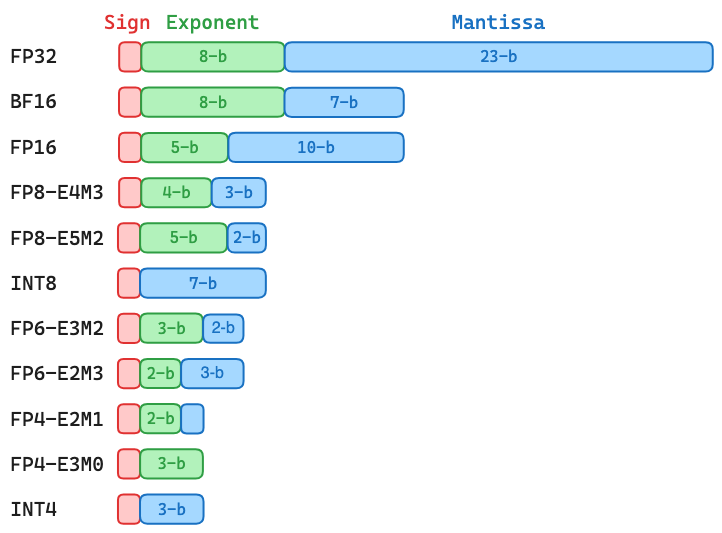
_{I-2. Floating-Point (FP)}

A floating-point representation is characterized by three components: Sign (S), Exponent (E), Mantissa (M). Since the sign always has a single bit, a floating-point representation with \(\mathrm{x}\)-bit exponent and \(\mathrm{y}\)-bit mantissa is often called \(\mathrm{\mathbf{ExMy}}\), which has the following binary pattern and decimal value:

\[\mathrm{S \; \underbrace{E_{x-1}\dots E_{0}}_{\text{Exponent}} \; \underbrace{M_{y-1}\dots M_{0}}_{\text{Mantissa}}} \,=\, \begin{cases} \,(-1)^{\,\mathrm{S}} \,\cdot\, \mathrm{2^{E-B} \,\cdot\, 1.{M}} & \text{if } \mathrm{E}\neq0 \\ \,(-1)^{\,\mathrm{S}} \,\cdot\, \mathrm{2^{1-B} \;\cdot\, 0.{M}} & \text{if } \mathrm{E}=0 \end{cases}\]

where \(\mathrm{E}\) and \(\mathrm{M}\) are interpreted as unsigned integers, the constant \(\mathrm{B = {2^{\,x-1}-1}}\) is a fixed “bias” that allows the actual exponent to be both positive and negative. Note that there is a leading bit before \(\mathrm{M}\), which makes the actual mantissa equal to \(1.{\mathrm{M}}\) or \(0.\mathrm{M}\). This leading bit is often called the hidden bit as it does not need to be stored. Instead, it can be determined during runtime by checking whether the value is normal \((\mathrm{E} \neq 0)\) or subnormal \((\mathrm{E} = 0)\).

For LLM training and inference, the default number representations are the 32-bit IEEE floating-point format (FP32-E8M23) and the 16-bit brain floating-point format (BF16-E8M7). In practice, BF16-E8M7 is often used to store model weights and activationsFor recent LLMs, BF16-E8M7 is often preferred over the 16-bit IEEE floating-point format (FP16-E5M10), because it has a wider dynamic range that helps prevent overflow during training., whereas FP32-E8M23 is used to store intermediate results of numerically sensitive operations (e.g., partial sums in dot product and softmax).

_{I-3. Hardware for INT and FP Arithmetic}

Given the importance of hardware efficiency for LLMs, it is useful to understand how a Multiply-Accumulate (MAC), the key operation in LLM training and inference, is carried out on hardware. Because a MAC consists of multiplication and addition, I will discuss the hardware implication of these two primitive operations under integer and floating-point representation.

_{Integer Addition and Multiplication}

The simplest integer adder is Ripple-Carry Adder, whose area and delay complexities ore \(\mathrm{O(N)}\)This bound assumes that a binary full-adder has a unit area and delay complexity of O(1). for \(\mathrm{N}\)-bit integer addition. Other adder architectures include Carry-Select Adder, Carry-Lookahead Adder, etc., which offer different trade-offs between area and delay.

The simplest integer multiplier multiplies every bits of two multiplicands via logical AND operations, followed by reducing these binary products via adder chains. This leads to an area complexity of \(\mathrm{O(N^2)}\) for \(\mathrm{N}\)-bit integer multiplication. Modern integer multipliers employ more efficient architectures, such as Wallace Tree and Dadda Tree, for fast reduction of binary products.

_{Floating-Point Multiplication}

The floating-point MAC is rather complicated as it needs to deal with exponent. To simply the discussion, I will only focus on normal floating-point numbers, whose binary exponent is larger than zero.

Consider two normal floating-point numbers \(\mathrm{F}_{1}\) and \(\mathrm{F}_{2}\,\):

\[\begin{aligned} \mathrm{F_1} \,&=\, (-1)^{\,\mathrm{S}_{1}} \,\cdot\, 2^{\mathrm{E}_{1}-\mathrm{B}} \,\cdot\, 1.\mathrm{M}_{1} \\ \mathrm{F_2} \,&=\, (-1)^{\,\mathrm{S}_{2}} \,\cdot\, 2^{\mathrm{E}_{2}-\mathrm{B}} \,\cdot\, 1.\mathrm{M}_{2} \end{aligned}\]

The multiplication product is:

\[\mathrm{P} = \mathrm{F_1} \cdot \mathrm{F_2} \,=\, (-1)^{\mathrm{S}_{1\,} \oplus\, \mathrm{S}_{2}} \,\cdot\, 2^{\mathrm{E}_{1} + \mathrm{E}_{2}-\mathrm{2B}} \,\cdot\, \underbrace{(\,1.\mathrm{M}_{1} \times 1.\mathrm{M}_{2}\,)}_{\text{Un-norm Mantissa}}\]

Based on the definition of floating-point representation as described previously, the sign, exponent, and mantissa of a product should be:

\[\begin{aligned} \mathrm{S_{P}} \,&=\, \mathrm{S}_{1} \oplus\, \mathrm{S}_{2} \\[0.3em] \mathrm{M_{P}} \,&=\, \begin{cases} \; (\,1.\mathrm{M}_{1} \times 1.\mathrm{M}_{2}\,) & \text{if un-norm mantissa} \leq 2 \\[0.1em] \;(\,1.\mathrm{M}_{1} \times 1.\mathrm{M}_{2}\,) \;/\; 2 & \text{if un-norm mantissa} > 2 \end{cases} \\[0.3em] \mathrm{E_{P}} \,&=\, \begin{cases} \;\mathrm{E}_{1} + \mathrm{E}_{2}-\mathrm{B} & \quad \text{if un-norm mantissa} \leq 2 \\[0.1em] \;\mathrm{E}_{1} + \mathrm{E}_{2}-\mathrm{B} + 1 & \quad \text{if un-norm mantissa} > 2 \\ \end{cases} \\ \end{aligned}\]

The above formula shows that:

• The product sign bit is simply a logical XOR between the sign bits of \(\mathrm{F}_{1}\) and \(\mathrm{F}_{2}\,\).
• The product mantissa can be obtained via unsigned integer multiplication between two input mantissa (\(1.\mathrm{M}_{1}\) and \(1.\mathrm{M}_{2}\)). A conditional check (a.k.a normalization) is needed to determine whether the un-normalized mantissa product is larger than 2. If yes, the un-normalized mantissa should be divided by 2, i.e., normalized to the range \([1, 2)\).
• The product exponent can be obtained via unsigned integer addition / subtraction between two input exponents (\(\mathrm{E}_{1}\) and \(\mathrm{E}_{2}\)) and the exponent bias (\(\mathrm{B}\))Note that we only subtract a single bias from (E₁ + E₂), since the standard floating-point representation will automatically subtract another exponent bias.. As discussed before, integer adder and multiplier have area complexity of \(\mathrm{O(N)}\) and \(\mathrm{O(N^2)}\), respectively. Since the cost of XORing the sign bit is negligible, the area complexity of a \(\mathrm{\mathbf{ExMy}}\) floating-point multiplier is roughly \(\mathrm{O(\,2x +(y+1)^2\,)}\). The following table shows the synthesized combinational logic area of BF16, FP16, and FP32 multipliers without the normalization stageIn a MAC unit, the normalization stage is placed after the accumulator., under 28nm technology. It can be observed that the area complexity offers a good estimation of the relative multiplier area across different floating-point representations.

Representation	Area Complexity	Multiplier Area
BF16-E8M7	80 (1×)	167.2 um2 (1×)
FP16-E5M10	131 (1.64×)	260.9 um2 (1.56×)
FP32-E8M23	592 (7.4×)	1166.8 um2 (6.98×)

_{Floating-Point Addition}

Again, consider two normal floating-point numbers \(\mathrm{F}_{1}\) and \(\mathrm{F}_{2}\,\):

\[\begin{aligned} \mathrm{F_1} \,&=\, (-1)^{\,\mathrm{S}_{1}} \,\cdot\, 2^{\,\mathrm{E}_{1}-\mathrm{B}} \,\cdot\, 1.\mathrm{M}_{1} \\ \mathrm{F_2} \,&=\, (-1)^{\,\mathrm{S}_{2}} \,\cdot\, 2^{\,\mathrm{E}_{2}-\mathrm{B}} \,\cdot\, 1.\mathrm{M}_{2} \end{aligned}\]

Let’s assume \(\mathrm{E}_{1} \geq \mathrm{E}_{2\,}\), then \(\mathrm{F}_{2}\) can be re-written as:

\[\mathrm{F_2} \,=\, (-1)^{\,\mathrm{S}_{2}} \,\cdot\, 2^{\,\mathrm{E}_{1}-\mathrm{B}} \,\cdot\, \left(\,1.\mathrm{M}_{2} \;/\; 2^{\,\mathrm{E}_{1}-\mathrm{E}_{2}}\,\right) \,=\, (-1)^{\,\mathrm{S}_{2}} \,\cdot\, 2^{\,\mathrm{E}_{1}-\mathrm{B}} \,\cdot\, \left(\,1.\mathrm{M}_{2} \gg (\mathrm{E}_{1}-\mathrm{E}_{2})\,\right)\]

The above step is called “Exponent Alignment”, where the two input exponents are compared and aligned to the larger one. Since we increase the exponent of \(\mathrm{F}_{2}\) by \((\,\mathrm{E}_{1}-\mathrm{E}_{2}\,)\), its mantissa needs to be divided by \(2^{\,\mathrm{E}_{1}-\mathrm{E}_{2}}\), which is equivalent to right-shifting the mantissa by \((\mathrm{E}_{1}-\mathrm{E}_{2})\) bits.

The addition sum can then be expressed as:

\[\mathrm{F_1} + \mathrm{F_2} \,=\, 2^{\,\mathrm{E}_{1} - \mathrm{B}} \,\cdot\, \underbrace{\left[\; (-1)^{\,\mathrm{S}_{1}} \cdot 1.\mathrm{M}_{1} \;+\; (-1)^{\,\mathrm{S}_{2}} \cdot \left(\,1.\mathrm{M}_{2} \gg (\mathrm{E}_{1}-\mathrm{E}_{2})\,\right) \;\right]}_{\text{Un-norm Mantissa}}\]

The sum’s sign and mantissa are derived from the above un-normalizaed mantissa through a hardware normalization block, which does some post-processing to ensure the final mantissa is normalized to the range \([1, 2)\).

Based on the above analysis, you may notice that it’s not straightforward to derive a good upper bound for the floating-point adder’s area complexity. There are also many low-level design considerations that vary across different hardware vendors when they design a floating-point adder. For example, how many bits should we reserve for accumulating the shifted mantissa \(1.\mathrm{M}_{2} \gg (\mathrm{E}_{1}-\mathrm{E}_{2})\) after exponent alignment? At FP32-E8M23, the largest and smallest representable exponents are \(127\) and \(-126\), respectively. This means that the 24-bit input mantissa (including the hidden bit) can be right-shifted by up to \(253\) bits, leading to a total precision of \(277\) bits for accumulating two aligned mantissa, which is clearly not a practical choice. Thus, in reality, the shifted mantissa is always truncated and accumulated with much lower precisionFor a given hardware platform, the exact precision of its mantissa accumulator can often be determined through reverse engineering.. This introduces a trade-off between numerical accuracy and hardware cost: allocating less precision to accumulate the shifted mantissa reduces hardware cost but harms numerical accuracyFor instance, DeepSeek-V3 finds that on NVIDIA H800 GPUs, the accumulation precision of FP8 MAC is only 14 bits, which can introduce a maximum relative error of nearly 2% compared to using FP32 accumulation precision..

II. Quantization Basics

Let’s now jump into quantization: one of the most popular methods to improve the hardware efficiency of LLMs.

_{II-1. Classification of Quantization Methods}

Before diving into technical details, I would like to classify existing quantization methods into two broad categories: compute-based and memory-based, depending on how they interpret the low-precision operands in hardwareThis is only one of many ways to classify quantization methods. For instance, one could also classify different methods based on their target quantized operands, e.g., weight-only quantization and weight-activation quantization, as described in this paper.. Below is a visualization:

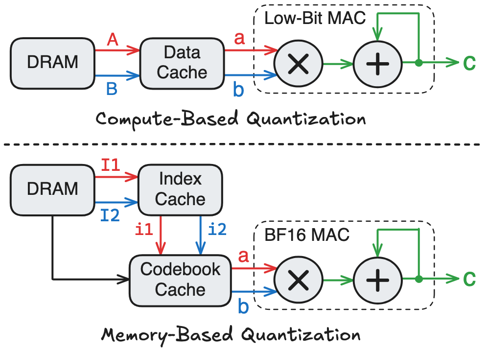
• Compute-based Quantization: The retrieved low-bit data from memory can be directly used to perform MAC. Examples include quantizing a tensor from BF16 to INT8 / FP8 / FP4, etc.
• Memory-based Quantization: The retrieved low-bit data from memory cannot be used to perform MAC. Instead, the low-bit data serves as an index to access another memory, which is often called a codebook and stores high-precision data (e.g., in BF16). The codebook access returns the actual data that is used to perform MAC.

Compute-based quantization enables computation on low-bit MAC hardware, whereas memory-based quantization requires an additional memory access to the codebook cache before performing computation on BF16 MAC hardware. Hence, at the same model compression ratio, compute-based quantization typically consumes significantly less area and energy, making it the favorable approach in modern LLMsExamples include DeepSeek-V3, DeepSeek-V4, Qwen3.5, etc. and AI chipsExamples include NVIDIA GPU, Meta MTIA, Tesla AI4, Microsoft MAIA, etc.. In the remaining of this blog, I will focus on discussing compute-based quantization.

_{II-2. Mathematical Background}

Given a tensor represented in high-precision floating-point (e.g., BF16), the purpose of quantization is to convert this tensor to a lower-precision format (e.g., INT8 / FP8), where every tensor element is mapped to its closest quantization value. However, directly mapping a high-precision number to a low-precision format can introduce many issues, such as overflow and underflow, which are illustrated below:

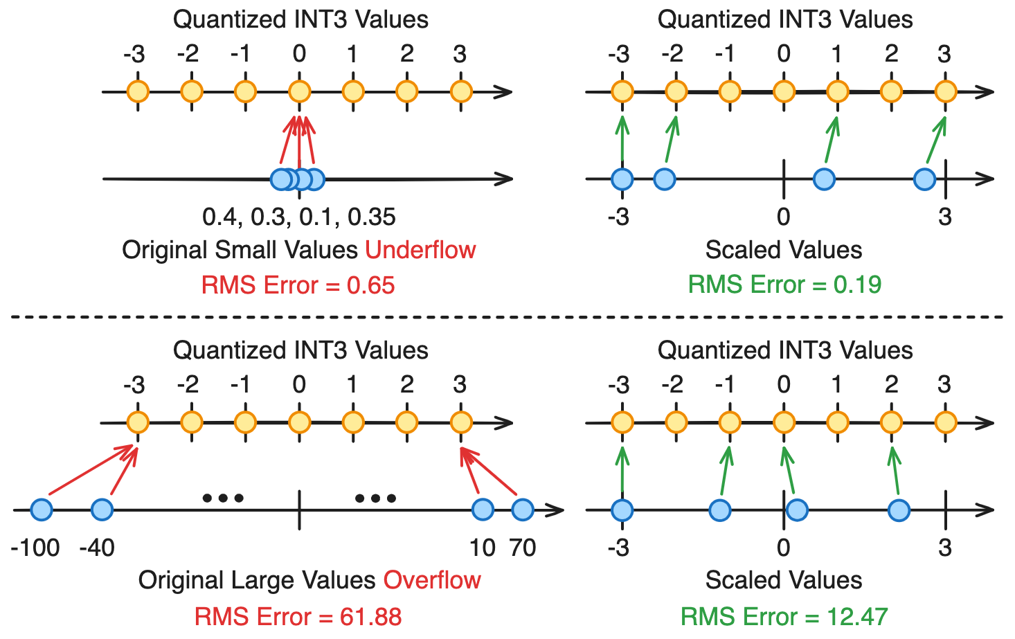
The above example quantizes a tensor of four elements to the 3-bit sign-magnitude integer (INT3) representation, and measures the resulting root-mean-square (RMS) quantization error. As shown in the top-left figure, if the original tensor contains very small values that are close to zero, directly casting to INT3 will make all values underflow to zero, resulting in catastrophic information loss. Similarly, as shown in the bottom left-figure, if the original tensor contains very large values that overflow the INT3 range, directly casting to INT3 will clamp these large values to the endpoint of INT3, resulting in significant saturation error.

To address the overflow and underflow issues, standard quantization linearly scales the original tensor to the quantized value range, then rounds each scaled tensor value to its nearest quantization value. After quantization, a re-scaling / dequantization step is performed at the end to map the quantized tensor back to the original tensor’s range. This procedure is summarized by the following equations:

\[\mathrm{S} = \frac{ |\mathrm{X}|_{\text{max}} }{ \mathrm{Q}_{\text{max}} } ; \ \ \ \mathrm{X_\mathrm{S}} = \frac{\mathrm{X}}{\mathrm{S}} ; \ \ \ \mathrm{X_Q} = \texttt{Round}\left(\,\mathrm{X_\mathrm{S}}\,,\, \mathrm{Q}\,\right) ; \ \ \ \mathrm{X_\mathrm{D}} = \mathrm{X_Q} \cdot \mathrm{S}\]

where \(\mathrm{X}\) is the original high-precision tensor, \(\mathrm{Q}\) is the set of quantization values defined by a low-bit number representation, \(\mathrm{S}\) is a high-precision scale factor, \(\mathrm{X_{S}}\) is the scaled tensor, \(\mathrm{X_{Q}}\) is the quantized tensor, and \(\mathrm{X_{D}}\) is the dequantized tensor. As shown in the above example, scaling can effectively mitigates the impact of overflow / underflow. When the tensor values are very small, scaling can enlarge the tensor range so that many elements are mapped to meaningful quantization values. When the tensor values are very large, scaling can prevent large saturation error.

Because of scaling, if two sets of quantization values, \(\mathrm{Q_{1}}\) and \(\mathrm{Q_{2}}\), differ only by a constant factor, then they produce mathematically equivalent results after dequantization:

\[\begin{aligned} \text{Assume}: \quad &\mathrm{Q_{2}} = c\,\mathrm{Q_{1}} \\[0.3em] \text{With }\mathrm{Q_{1}}: \quad & \mathrm{S_{1}} = \frac{ |\mathrm{X}|_{\text{max}} }{ \mathrm{Q}_{1,\text{max}} } ; \ \ \mathrm{X_{S_{1}}} = \frac{\mathrm{X}}{\mathrm{S_{1}}} ; \ \ \mathrm{X_{Q_{1}}} = \texttt{Round}\left(\mathrm{X_{S_{1}}}, \mathrm{Q_{1}}\right) ; \ \ \mathrm{X_{D_{1}}} = \mathrm{X_{Q_{1}}} \cdot \mathrm{S_{1}} \\[0.3em] \text{With }\mathrm{Q_{2}}: \quad & \mathrm{S_{2}} = \frac{ \mathrm{S_{1}} }{ c } ; \ \ \mathrm{X_{S_{2}}} = \frac{c\,\mathrm{X}}{\mathrm{S_{1}}} ; \ \ \mathrm{X_{Q_{2}}} = \texttt{Round}\left(c\,\mathrm{X_{S_{1}}}, \mathrm{c\,Q_{1}}\right) = c\,\mathrm{X_{Q_{1}}} ; \ \ \mathrm{X_{D_{2}}} = \mathrm{X_{Q_{2}}} \cdot \mathrm{S_{2}} = \mathrm{X_{D_{1}}} \\[0.3em] \end{aligned}\]

For example, at 4-bit quantization, you might have seen some papers using a format called E1M2, which has the set of quantization values \(\pm\{\,0,\, 0.25,\, 0.5,\, 0.75,\, 1,\, 1.25,\, 1.5,\, 1.75\,\}\). This is actually equivalent to INT4 quantization with the set of values \(\pm\{\,0,\, 1,\, 2,\, 3,\, 4,\, 5,\, 6,\, 7\,\}\).

_{II-3. Hardware Benefits of Quantized GEMM}

By reducing the operand bit-width, quantization not only decreases the memory footprint, but also enables more efficient computation on low-precision MAC hardware. When the baseline LLM stores model weights and input activations in BF16, its linear layer will perform a GEMM using BFP16 multiply and FP32 accumulation. As an example, if we employ per-tensor quantization to convert model weights and input activations to INT8, the linear layer can instead perform a GEMM using INT8 multiply and INT32 accumulation, followed by dequantization that multiplies the output matrix with two scale factors. This is visualized below:

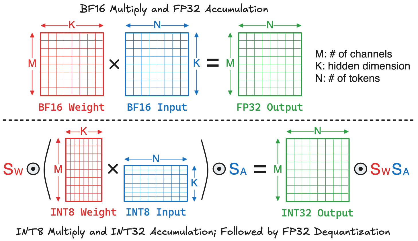
To understand the hardware implication of these two approaches, we can break down the hardware cost into two parts: memory and computation. The memory can be quantified as the total number of bytes required to store weights, inputs, and outputs. Accordingly, the memory costs of baseline and quantized GEMMs are:

\[\begin{aligned} \text{Baseline:} & \ \ 2MK + 2KN + 4MN \\ \text{Quantized:} & \ \ MK + KN + 4MN \end{aligned}\]

For computation, recall that a GEMM with size \(M\times K \times N\) requires \(MKN\) MAC operations. For dequantization, the scale factors \(\mathrm{S_{W}}\) and \(\mathrm{S_{A}}\) can be pre-multiplied and stored as a constant. Multiplying this constant with the output matrix requires \(MN\) multiplications. Thus, the computation costs of baseline and quantized GEMMs are:

\[\begin{aligned} \text{Baseline:} & \ \ MKN \cdot \text{MAC}_{\text{BF16-FP32}} \\ \text{Quantized:} & \ \ MKN \cdot \text{MAC}_{\text{INT8-INT32}} \,+\, (MN+1) \cdot \text{MUL}_{\text{FP32}} \end{aligned}\]

In modern LLMs, the \(K\)-dimension is usually very large (e.g., several thousands), making the cost of dequantization negligible compared to MAC. Consequently, the compute cost is roughly proportional to the cost of MAC units. The following table summarizes the synthesized area and energy of MAC units at different input-output precisions under 28nm technology. It can be observed that integer quantization can significantly reduce the computation cost compared to high-precision floating-point operationsIn some cases, a quantization strategy chooses to maintain the original 16-bit precision to avoid unacceptable accuracy loss, and instead uses a more hardware-efficient number representation to reduce the computation cost. For instance, INT16 does not save memory cost over BF16, but it can reduce the area and energy of MAC by ~1.8×..

Multiplier	Accumulator	Area (um2)		Energy (pJ)
		Value	Ratio	Value	Ratio
INT8	INT32	213.8	1×	0.16	1×
INT8	INT48	286.2	1.34×	0.22	1.38×
INT16	INT48	516.2	2.41×	0.36	2.25×
BF16	FP32	929.4	4.35×	0.63	3.94×
FP32	FP32	1994.7	9.33×	1.28	8×

III. Advanced Quantization Techniques

In this section, I will discuss several techniques for improving the performance of quantized LLM inference. Many of these techniques are widely adopted in SoTA LLMs and AI chips. From an algorithm-hardware co-design perspective, a good quantization strategy introduces a trade-off between model accuracy, memory footprint, and computational efficiency. These trade-offs will also be examined throughout this section.

_{III-1. Block-Wise Quantization}

Block-wise quantization is employed in many recent LLMs such DeepSeek-V3, GPT-OSS, and Kimi-K2. Before diving into this technique, let’s first understand the concept of outliers. An outlier is defined as a value whose magnitude is significantly larger than the rest of values in a tensor. It is well known that LLM tensors contain extreme outliers, and preserving the numerical fidelity of these outliers is the key to reducing quantization error and improving model performanceFor more details, interested readers can checkout this paper..

Quantization granularity measures how many elements are scaled and quantized together. For example, the coarsest quantization granularity is simply Tensor-Wise Quantization. But at this granularity, even a single outlier can significantly squeeze most of the remaining values, making them underflow to zero after quantization. This phenomenon is visualized in the following top-left figure, which uses INT4 sign-magnitude representation to quantize a \(3\times4\) tensor. To mitigate the impact of outliers, we can reduce the quantization granularity so that fewer values are quantized together. For example, Row-Wise Quantization applies independent scaling to each row of a tensor, limiting the effect of an outlier to values within the same row, as illustrated in the following top-right figure. On top of row-wise quantization, the granularity can be further reduced by partitioning each row into smaller segments / blocks, an approach called Block-Wise Quantization, which further constrains the impact of outliers to a small block. This is illustrated in the following bottom figure, where a row is partitioned into two blocks:

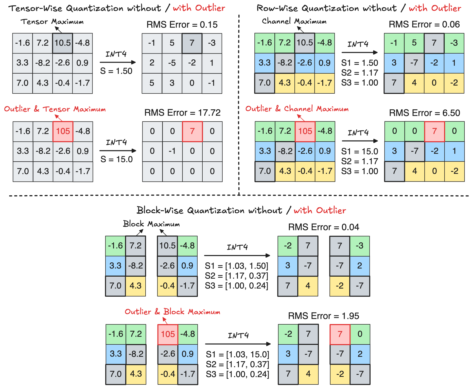
Why Does Block-Wise Quantization Help? Let’s analyze how quantization affects the maximum element \(\mathrm{X}_{\text{max}}\)Here, the "maximum element" refers to the element with maximum magnitude, thus can be either positive or negative., without caring about granularity. In addition, let’s assume the quantized number representation is symmetric with respect to zero (i.e., \(\mathrm{Q}_{\text{max}} = -\mathrm{Q}_{\text{min}}\,\)), which holds for most number representations such as floating-point and sign-magnitude integer. According to the definition of quantization, we have:

\[\begin{aligned} \mathrm{S} &= \frac{ |\mathrm{X}|_{\text{max}} }{ \mathrm{Q}_{\text{max}} } = \frac{ |\mathrm{X}_{\text{max}}| }{ \mathrm{Q}_{\text{max}} } \\[0.3em] \mathrm{X_{\text{max},\,S}} &= \frac{ \mathrm{X}_{\text{max}}}{\mathrm{S}} = \frac{ \mathrm{X}_{\text{max}}\cdot \mathrm{Q}_{\text{max}} }{ |\mathrm{X}_{\text{max}}| } = \mathrm{X}_\text{sign} \cdot \mathrm{Q}_{\text{max}} \\[0.3em] \mathrm{X_{\text{max},\,Q}} &= \texttt{Round-To-Nearest}\left(\,\mathrm{X_{\text{max},\,S}}\,,\, \mathrm{Q}\,\right) = \mathrm{X}_\text{sign} \cdot \mathrm{Q}_{\text{max}} \\[0.3em] \mathrm{X_{\text{max},\,D}} &= \mathrm{X_{\text{max},\,Q}} \cdot \mathrm{S} = \left(\,\mathrm{X}_\text{sign} \cdot \mathrm{Q}_{\text{max}}\,\right) \,\cdot\, \frac{ |\mathrm{X}_{\text{max}}| }{ \mathrm{Q}_{\text{max}} } = \mathrm{X}_{\text{max}} \end{aligned}\]

The above last equation unveils a critical insight: If the scale factor is accurately computed (e.g., using high precision such as FP32), then the original maximum element remains unchanged after dequantization, regardless of the quantization granularity. In other words, the maximum element of a granularity has no quantization error. Therefore, under a finer quantization granularity, more maximum elements can be represented accurately, leading to lower total quantization error.

Algorithm-Hardware Trade-Off under Different Granularity: As discussed above, an obvious benefit of reduced quantization granularity is lower quantization error, which potentially offers better model accuracy. However, this algorithmic benefit comes with additional computation and memory costs. Below, I try to visualize the computation flow of performing a \(M\times K \times N\) GEMM under different INT4 quantization granularity:

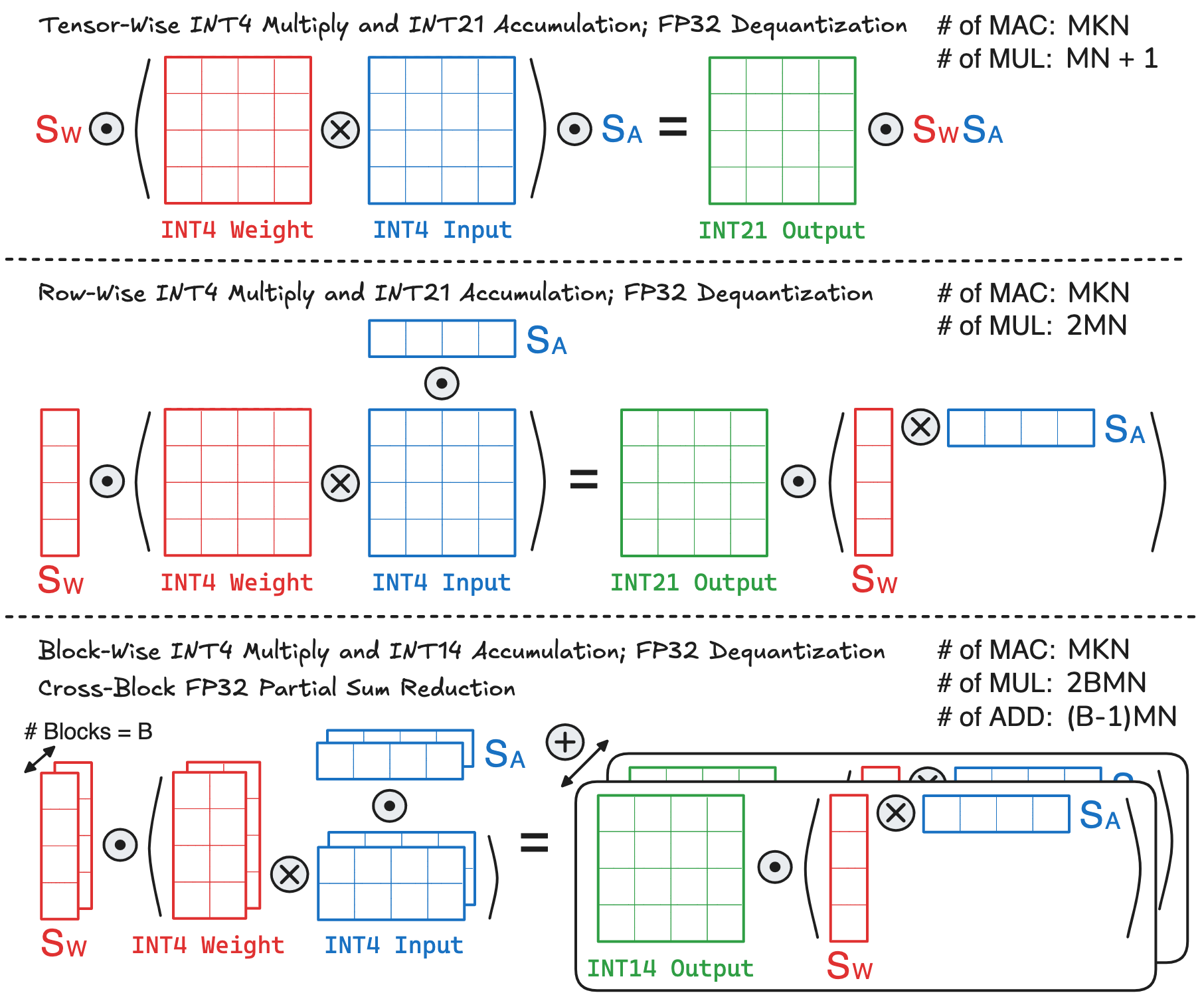
• Tensor-Wise Quantization: This is the coarsest granularity, where the GEMM requires \(MKN\) low-precision MAC operations. For dequantization, the FP32 scale factors \(\mathrm{S_{W}}\) and \(\mathrm{S_{A}}\) can be pre-multiplied and stored as a constant, and multiplying this constant with the output matrix requires \(MN\) FP32 multiplications.
• Row-Wise Quantization: The whole GEMM still requires \(MKN\) low-precision MAC operations. But for dequantization, the row-wise scale factors of weight and activation are vectors of size of \(M \times 1\) and \(N \times 1\), respectively. These two vectors first perform an outer product, which is then element-wise multiplied with the output matrix, leading to \(2MN\) FP32 multiplications.
• Block-Wise Quantization: Since a matrix row is partitioned into multiple blocks, the complete row-wise dot product will contain \(B\) partial sums, where \(B\) is the number of blocks. This means that the whole GEMM is partitioned into \(B\times\) small GEMMs, each of size \((M \times K/B \times N)\) with row-wise quantization (a block of the original large GEMM can be viewed as a row of the small GEMM). The total number of low-precision MAC operations remains \(B \times (M \times K/B \times N) = MKN\). The tricky part comes to the dequantization process: every small GEMM requires \(2MN\) multiplications as in row-wise quantization, leading to a total of \(2BMN\) FP32 multiplications. But the dequantized output matrix of every small GEMM only forms a partial sum, which also needs to be reduced over all blocks, leading to a total of \((B-1)MN\) extra FP32 additions.

One thing I didn’t explain in the above figure, which you might find a little weird, is the output matrix precision. When I talk about BF16 GEMM and INT8 GEMM in previous sections, I used FP32 and INT32 as the output precision. However, the output matrix precision can be reduced according to the input precision, which in turn reduces the hardware accumulator precision and cost. Taking the above example, the sign-magnitude INT4 representation has a numerical range of \([-7, 7]\), and multiplying two INT4 numbers yields a range of \([-49, 49]\). Consider a trillion-parameter LLM such as Kimi-K2.5, whose maximum dot product size of \(18432\). Under tensor-wise and row-wise INT4 quantizationHere, I am only using Kimi-K2.5 as an illustrative example to describe how we can optimize the hardware accumulator precision considering the quantization precision and dot product size. In practice, Kimi-K2.5 keeps input activations in BF16 and applies INT4 block-wise quantization to weights. More generally, tensor-wise or row-wise quantization is rarely used at very low precisions such as 4 bits., the INT4 dot product output has a range of \([-903168, 903168]\), which can be represented with a 21-bit sign-magnitude integerIn practice, the output accumulator precision may be further optimized depending on the data statistics, as it's impossible that all quantized INT4 values are -7 and 7.. Similarly, for block-wise INT4 quantization under a typical block size of 128, the dot product output has a range of \([-6272, 6272]\), which can be represented with a 14-bit sign-magnitude integer.

The memory costs of different quantization granularity are much simpler to analyze. In addition to weight, input, and output, quantization stores extra metadata such as the scale factors. For tensor-wise and row-wise quantization, the memory cost of scale factors is pretty negligible when the dot product size is large enough, which is the case for modern LLMs. However, this assumption may not hold for block-wise quantization. For example, with a block size of \(128\), an FP32 scale factor introduces an overhead of \(32/128 = 0.25\) bits per element. As the block size further decreases (to improve model performance), the storage overhead of scale factors can no longer be ignored. Thus, for the next quantization technique, I will discuss how to reduce the overhead of scale factors.

_{III-2. Scale Factor Quantization}

While block-wise quantization brings algorithmic benefits by reducing quantization error, it incurs additional hardware cost from storing numerous FP32 scale factors and performing more FP32 multiplications / additions during dequantization. This overhead restricts the use of very small block sizes, which are often critical for achieving high accuracy under 4-bit quantization.

The question is: How can we reduce the cost of scale factors? The answer is surprisingly straightforward: if quantization can reduce the memory and computation costs of tensor elements, why not apply it to scale factors? Building on this idea, the industry has proposed two methods to quantize the block scale: Microscaling (MX) and NVIDIA’s (NV) approach. Both quantize the scale factor to 8 bits, but using different number representationsBesides the scale factor representation, the official MX and NV quantization recipe also set fixed block sizes of 32 and 16, respectively. However, the concept of block size is not strictly tied to these two approaches. For instance, one can choose to reduce the MX block size from 32 to 16, as did in this paper from Meta. Therefore, I will focus on discussing the scale factor representation without caring too much about the block size.: MX uses the 8-bit power-of-two format (E8M0), whereas NV uses the 8-bit floating-point format with 4-bit exponent and 3-bit mantissa (FP8-E4M3). Below is a visualization of how MX and NV represent scale factors, assuming the block elements are quantized to FP4 (i.e., the popular MXFP4 and NVFP4 formats):

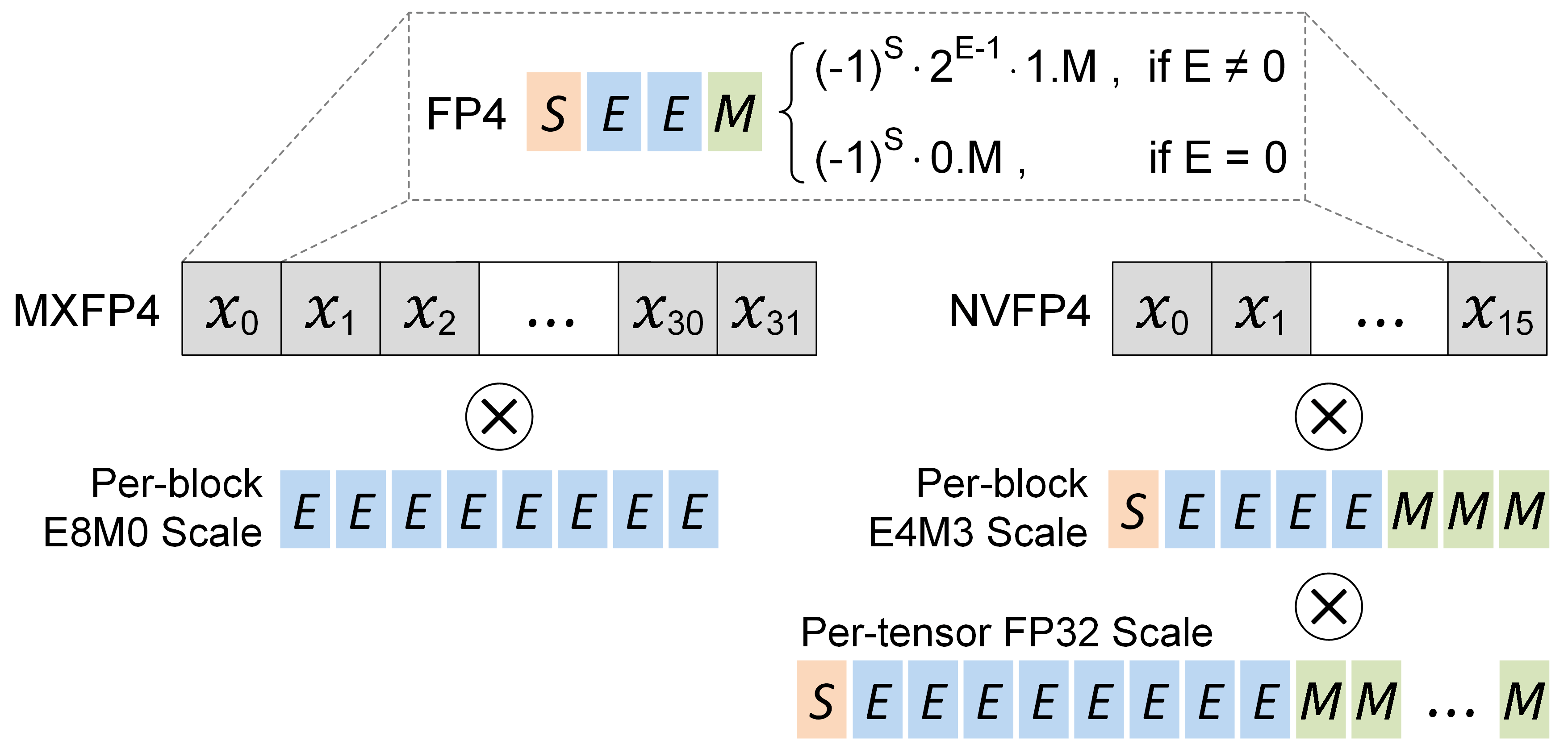
_{Microscaling (MX)}

MX is standardized by the Open Compute Project, and widely supported by recent AI chips such as AMD Radeon, Meta MTIA, and Microsoft MAIA. In this approach, the high-precision scale factor is quantized to an 8-bit power-of-two (E8M0). For example, the widely used MXFP4 quantization scheme can be expressed by the following equationsThis is also applicable to other MXFP formats such as MXFP8, as described in this paper.:

\[\mathrm{S} = \frac{ |\mathrm{B}|_{\text{max}} }{ \mathrm{Q}_{\text{max}} } ; \ \ \mathrm{S_{Q}} = 2^{\left\lceil\,\texttt{log2}\left( \,\mathrm{S} \,\right) \,\right\rceil} ; \ \ \mathrm{B_S} = \frac{\mathrm{B}}{\mathrm{S_{Q}}} ; \ \ \mathrm{B_Q} = \texttt{Round}\left(\,\mathrm{B_S}\,,\, \text{FP4}\,\right) ; \ \ \mathrm{B_D} = \mathrm{B_Q} \cdot \mathrm{S_{Q}}\]

where \(\mathrm{B}\) is the block to be quantized, and \(\mathrm{Q}_{\text{max}} = 6\) is the maximum FP4 quantization value. After calculating the scale factor \(\mathrm{S}\), we take its binary logarithm followed by a ceiling operation to obtain the integer exponentWhen implementing this step in code, there is no need to explicitly compute the logarithm, which is very costly on hardware. Instead, this whole step can be efficiently implemented at the binary level using simple bitwise operations, as described in this code snippet from DeepSeek.. The quantized scale factor is the base-2 exponentiation of this integer exponent. The ceiling operation ensures that \(\mathrm{S}\) is always rounded up to the nearest power-of-two that is larger than or equal to \(\mathrm{S}\). This is different from the rounding mechanism for the scaled block element \(\mathrm{B_{S}\,}\), which is rounded (up or down) to the nearest quantization value.

The purpose of rounding up during the power-of-two scale factor quantization in MXFP4, is to ensure the scaled block \(\mathrm{B_{S}}\) can always remains within the representable quantization range without significant overflow. Specifically, we want to ensure that:

\[\begin{aligned} |\mathrm{B_{S}}| \leq \mathrm{Q}_{\text{max}} \iff |\mathrm{B_{\text{max},\,S}}| \leq \mathrm{Q}_{\text{max}} \iff \frac{|\mathrm{B_{\text{max}}}|}{\mathrm{S_{Q}}} \leq \mathrm{Q}_{\text{max}} \iff \mathrm{S_{Q}} \geq \frac{|\mathrm{B_{\text{max}}}|}{\mathrm{Q}_{\text{max}}} \iff \mathrm{S_{Q}} \geq\, \mathrm{S} \end{aligned}\]

Interested readers may ask: Why don’t we use the normal rounding (up or down) mechanism when rounding the scale factor to its nearest power-of-two? In fact, this is exactly what the original MXFP4 quantizer from Microsoft does when the block maximum’s mantissa exceeds the quantization maximum’s mantissaIn the original MXFP4 quantizer from Microsoft, the power-of-two block scale of MXFP4 is computed as $$\mathrm{S_{Q, \,\text{MXFP4}}} = 2^{\left\lfloor\,\texttt{log2}\left(\mathrm{B_{\text{max}}}\right)\,\right\rfloor \,-\, 2}$$. However, this naive approach may cause significant overflow of the scaled block \(\mathrm{B_{S}\,}\), leading to large saturation error for MXFP4 quantizationHence, you should never refer to that original implementation for MXFP4 quantization. But you can refer to that for some MX formats such as MXINT4 quantization, whose quantized E8M0 scale is also computed as $$\mathrm{S_{Q, \,\text{MXINT4}}} = 2^{\left\lfloor\,\texttt{log2}\left(\mathrm{B_{\text{max}}}\right)\,\right\rfloor \,-\, 2}$$You may want to think why the MXINT4 scale can be quantized in this way even overflow occurs when the mantissa is larger than 1.75. To better explain this problem, lLet’s analyze what happens to the block maximum, \(\mathrm{B}_{\text{max}\,}\), when the scale factor is rounded (up or down) to its nearest power-of-two. For simplicity, I will assume \(\mathrm{B}_{\text{max}}\) is a positive normal FP32 value, leading to the following equations for computing the scaled block maximum:

\[\mathrm{S} = \frac{\mathrm{B}_{\text{max}}}{6} ; \ \ \mathrm{S_{Q}} = 2^{\left\lfloor\,\texttt{log2}\left( \,\mathrm{S} \,\right) \,\right\rceil} ; \ \ \mathrm{B_{\text{max},\,S}} = \frac{\mathrm{B}_{\text{max}}}{\mathrm{S_{Q}}}\]

Since \(\mathrm{B}_{\text{max}}\) is a positive normal FP32 value, I can write it in floating-point representation as described in Section I-2:

\[\mathrm{B_{\text{max}}} = 0\;\mathrm{\underbrace{E_{7}\dots E_{0}}_{\text{Exponent}} \; \underbrace{M_{22}\dots M_{0}}_{\text{Mantissa}}} = (-1)^0 \cdot 2^{\mathrm{E}-127} \cdot (\,1+\mathrm{M}\,) = 2^{\mathrm{E\,'}} \cdot \mathrm{M\,'}\]

where \(\mathrm{E\,'}\) is the actual exponent after subtracting the bias \(127\), and \(\mathrm{M\,'}\) is the actual mantissa after adding the hidden bit \(1\) for normal values. Using this representation, the scale factor can be expressed as:

\[\mathrm{S} = \frac{\mathrm{B}_{\text{max}}}{6} = \frac{ 2^{\,\mathrm{E\,'}} \cdot \mathrm{M\,'} }{ 2^2 \cdot 1.5 } = 2^{\,\mathrm{E\,'} - \,2} \cdot \frac{\mathrm{M\,'}}{1.5}\]

Now, consider the 50% case where \(\mathrm{M\,'} > 1.5\)Assume the block maximum's mantissa is uniformly distributed between [1, 2), then we have a high probability of 50% that it exceeds 1.5, and because \(\mathrm{M\,'} < 2\) by definition of the floating-point representation, we have:

\[\begin{aligned} & 2^{\,\mathrm{E\,'} - \,2} \cdot \frac{1.5}{1.5} \,<\, \mathrm{S} \,<\, 2^{\,\mathrm{E\,'} - \,2} \cdot \frac{2}{1.5} \\[0.3em] \iff\; & \mathrm{E\,'} - 2 \,<\, \texttt{log2}\left( \,\mathrm{S} \,\right) \,<\, \mathrm{E\,'} - 2 + 0.415 \\[0.3em] \implies\; & \left\lfloor\,\texttt{log2}\left(\,\mathrm{S} \,\right) \,\right\rceil \,=\, \mathrm{E\,'} - 2 \\[0.3em] \implies\; & \mathrm{S_{Q}} \,=\, 2^{\left\lfloor\,\texttt{log2}\left(\,\mathrm{S} \,\right) \,\right\rceil} \,=\, 2^{\mathrm{E\,'} - 2} \\ \implies\; & \mathrm{B_{\text{max},\,S}} \,= \frac{\mathrm{B}_{\text{max}}}{\mathrm{S_{Q}}} =\, \frac{2^{\mathrm{E\,'}} \cdot \mathrm{M\,'}}{2^{\mathrm{E\,'} - 2}} = \, 4\,\mathrm{M\,'} \in\, (\,6,\,8\,) \\[0.3em] \implies\; & \mathrm{B_{\text{max},\,Q}} = \texttt{Round}\left(\,\mathrm{B_{\text{max},\,S}}\,,\, \text{FP4}\,\right) = 6 \end{aligned}\]

The above derivation implies that: If the mantissa of \(\mathrm{B}_{\text{max}}\) is larger than 1.5, then \(\mathrm{B_{\text{max},\,S}}\) will overflow outside the FP4 rangeThe above analysis can be generalized to other number representations under MX quantization: If the mantissa of B_max is larger than the mantissa of Q_max (e.g., 1.5 for FP4), then rounding (up or down) the scale factor to its nearest power-of-two will cause B_{max, S} to overflow outside the representable quantization range.. Consequently, the quantized block maximum, \(\mathrm{B_{\text{max},\,Q\,}}\), is always mapped / clamped to the largest representable FP4 value, \(6.0\), leading to saturation error. On the other hand, if we only round up the scale factor to its nearest power-of-two, we have:

\[\begin{aligned} & 2^{\,\mathrm{E\,'} - \,2} \cdot \frac{1.5}{1.5} \,<\, \mathrm{S} \,<\, 2^{\,\mathrm{E\,'} - \,2} \cdot \frac{2}{1.5} \\[0.3em] \iff\; & \mathrm{E\,'} - 2 \,<\, \texttt{log2}\left( \,\mathrm{S} \,\right) \,<\, \mathrm{E\,'} - 2 + 0.415 \\[0.3em] \implies\; & \left\lceil\,\texttt{log2}\left( \,\mathrm{S} \,\right) \,\right\rceil \,=\, \mathrm{E\,'} - 1 \\[0.3em] \implies\; & \mathrm{S_{Q}} \,=\, 2^{\left\lceil\,\texttt{log2}\left( \,\mathrm{S} \,\right) \,\right\rceil} \,=\, 2^{\mathrm{E\,'} - 1} \\ \implies\; & \mathrm{B_{\text{max},\,S}} \,= \frac{\mathrm{B}_{\text{max}}}{\mathrm{S_{Q}}} =\, \frac{2^{\mathrm{E\,'}} \cdot \mathrm{M\,'}}{2^{\mathrm{E\,'} - 1}} = \, 2\,\mathrm{M\,'} \in\, (\,3,\,4\,) \\[0.3em] \implies\; & \mathrm{B_{\text{max},\,Q}} = \texttt{Round}\left(\,\mathrm{B_{\text{max},\,S}}\,,\, \text{FP4}\,\right) = 3 \,\ \text{or} \,\ 4 \end{aligned}\]

Now, \(\mathrm{B_{\text{max},\,Q}}\) can be mapped to two representable FP4 values: \(3\) or \(4\), whichever is closer to \(\mathrm{B_{\text{max},\,S}}\). This offers more flexibility compared to the naive rounding mechanism, where \(\mathrm{B_{\text{max},\,Q}}\) can only be mapped / clamped to \(6\).

The above analysis also indicates a hardware-efficient strategy for calculating the block scale of MXFP4:

if (B_max.man > 1.5):
  block_exp = B_max.exp - 1 
else: # (B_max.man <= 1.5)
  block_exp = B_max.exp - 2

block_scale = 2 ** block_exp

which completely eliminates the division (\(\mathrm{B_{\text{max}}}\,/\,6\)), logarithm, and ceiling operations to compute the block scale. Assume the block element is represented in BF16-E8M7, then a SystemVerilog implementation can be:

input  logic [15:0] B_max;
output logic [8:0]  block_exp;
output logic [15:0] block_scale;

always_comb begin
  if (B_max[6:0] > 7'b1000000) // Think why this is equivalent to (B_max.man > 1.5)
      block_exp = B_max[14:7] - 1 
  else
      block_exp = B_max[14:7] - 2
end

assign block_scale = {1'b0, block_exp, 7'd0};

To measure the algorithmic performance of MX under the two rounding approaches for scale factor quantization, I implement the naive MXFP4 quantizer and the enhanced MXFP4 quantizer. The following table shows the perplexityPerplexity is a widely used metric to quantify the LLM performance, and lower perplexity means better performance. of Wikitext-2 dataset on several Llama3 and Qwen3 models, under MXFP4 weight-activation quantization with a block size of 16. The round-up approach achieves much better perplexity compared to the naive round-to-nearest approach for power-of-two scale factor quantization.

	Llama-3.1-8B	Llama-3.2-3B	Qwen3-4B	Qwen3-8B
Naive Round	9.51	15.35	17.46	11.84
Round-Up	8.69	13.58	15.69	10.66

_{NVIDIA’s (NV) Approach}

Recall from Section III-1, if the scale factor is accurately represented (e.g., in FP32), then the maximum element can be accurately quantized without error. However, the E8M0 scale factor used in MX violates this condition and introduces error for the block’s maximum elementAgain, the "maximum element" refers to the element with maximum magnitude.. This raises the question: Can we minimize the quantization error of block maximum while still using an 8-bit scale factor?

Let’s try to understand the limitations of MX when quantizing the block maximum, \(\mathrm{B}_{\text{max}}\). Again, for simplicity, assume \(\mathrm{B}_{\text{max}}\) is a positive normal FP32 value:

\[\mathrm{B_{\text{max}}} = 0\;\mathrm{\underbrace{E_{7}\dots E_{0}}_{\text{Exponent}} \; \underbrace{M_{22}\dots M_{0}}_{\text{Mantissa}}} = (-1)^0 \cdot 2^{\mathrm{E}-127} \cdot (\,1+\mathrm{M}\,) = 2^{\mathrm{E\,'}} \cdot \mathrm{M\,'}\]

Since the scale factor of MX is power-of-two, scaling \(\mathrm{B}_{\text{max}}\) will only change its exponent without affecting mantissa:

\[\mathrm{B_{\text{max},\,S}} \,= \frac{\mathrm{B}_{\text{max}}}{\mathrm{S_{MX}}} \,= \frac{2^{\mathrm{E\,'}} \cdot \mathrm{M\,'}}{\mathrm{S_{MX}}} = \, 2^{\widetilde{\mathrm{E}}} \cdot \mathrm{M\,'}\]

Comparing the above result with the case of accurate FP32 scaling:

\[\mathrm{S}_{\text{FP32}} = \frac{ \mathrm{B}_{\text{max}} }{ \mathrm{Q}_{\text{max}} }; \ \ \ \mathrm{B_{\text{max},\,S}} = \frac{ \mathrm{B}_{\text{max}}}{\mathrm{S}_{\text{FP32}}} = \mathrm{Q}_{\text{max}}\]

We observe the accurate scaling gives \(\mathrm{B_{\text{max},\,S}} = \mathrm{Q}_{\text{max}\,}\), which implies the mantissa of \(\mathrm{B_{\text{max},\,S}}\) is equal to that of \(\mathrm{Q}_{\text{max}}\) (e.g., \(1.5\) for FP4). However, under MX scaling, the mantissa of \(\mathrm{B_{\text{max},\,S}}\) is equal to that of \(\mathrm{B_{\text{max}}\,}\), which can take any value in \([\,1.0,\, 2.0\,)\). Consequently, MX can be viewed as effectively quantizing the mantissa of \(\mathrm{B_{\text{max}}}\) to the representable mantissa of \(\mathrm{Q}\)For example, with the MXFP4 quantization described just now, B_max can be quantized to 3, 4, or 6. These three quantization values have two mantissa, 1.0 and 1.5, which are the representable mantissas of FP4., resulting in quantization error on \(\mathrm{B}_{\text{max}}\). To reduce this error, one approach is to make the mantissa of \(\mathrm{B_{\text{max}}}\) closer to that of \(\mathrm{Q}_{\text{max}}\) through additional mantissa scaling, which requires the scale factor to also contain mantissa bitsFor example, assume B_max = 2^E' × M' has a mantissa M' = 1.875. Under MXFP4 quantization, S = 2^{E' - 1} and B_{max, S} = 3.75 will be rounded to 4, leading to an error of 0.25. But if S can store a 2-bit mantissa, then S = 2^{E' - 2} × 1.25 and B_{max, S} = 6 can be accurately quantized without error.

Building on this insight, NVIDIA (NV) proposes to employ FP8-E4M3, the 8-bit floating-point format with 4-bit exponent and 3-bit mantissa, for block scale quantization, as described in the following equations:

\[\begin{aligned} &\mathrm{S} = \frac{ |\mathrm{B}_{\text{max}}| }{ \mathrm{Q}_{\text{B,max}} } \\[0.3em] &\mathrm{S'} = \frac{ \mathrm{S}_{\text{max}} }{ \mathrm{Q}_{\text{S,max}} } = \left(\frac{ |\mathrm{B}_{\text{max}}| }{ \mathrm{Q}_{\text{B,max}}}\right)_{\text{max}} \cdot \frac{1}{\mathrm{Q}_{\text{S,max}} } = \frac{|\mathrm{B}_{\text{max}}|_{\text{max}}}{\mathrm{Q}_{\text{B,max}}} \cdot \frac{1}{\mathrm{Q}_{\text{S,max}}} = \frac{|\mathrm{T}_{\text{max}}|}{\mathrm{Q}_{\text{B,max}} \cdot\mathrm{Q}_{\text{S,max}}} \\[0.3em] &\mathrm{S_S} = \frac{\mathrm{S}}{\mathrm{S'}} \\[0.3em] &\mathrm{S_Q} = \texttt{Round}\left(\,\mathrm{S_S}\,,\, \text{FP8}\,\right) \\[0.3em] &\mathrm{S_\mathrm{D}} = \mathrm{S_Q} \cdot \mathrm{S'} \end{aligned}\]

where \(\mathrm{Q}_{\text{B,max}}\) is the maximum quantization value for the block element, \(\mathrm{Q}_{\text{S,max}}\) is the maximum quantization value for the block scale (i.e., \(448\) for FP8), \(\mathrm{S}'\) is the scale of block scale, \(\mathrm{T}_{\text{max}}\) is the tensor maximum, \(\mathrm{S_{S}}\) is the scaled block scale, \(\mathrm{S_{Q}}\) is the quantized block scale, and \(\mathrm{S_{D}}\) is the final dequantized block scale. This block scale quantization process is exactly the same as how we quantize a tensor as discussed in Section II-2. The mathematical equations are therefore also the same as those for tensor quantization, except that we change \(\mathrm{X}\) to \(\mathrm{S}\), \(\mathrm{S}\) to \(\mathrm{S'}\), and \(\mathrm{Q}\) to FP8. Below is a visualization to help you understand the FP8 block scale quantization using the popular NVFP4 format (i.e., \(\mathrm{Q}_{\text{B,max}}\) = 6) as an example.

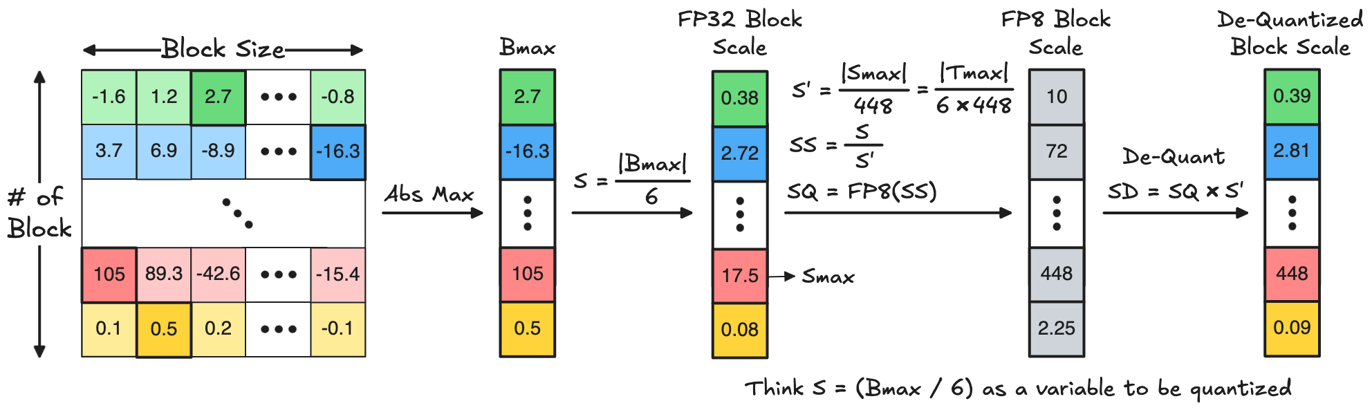
The above equation for calculating \(\mathrm{S'}\) indicates a tensor-wise scaling, as also described in NVIDIA’s blogPersonally, I find NVIDIA’s description of tensor-wise scaling somewhat vague; hopefully, my explanation provides greater clarity.. The reason is that, when following the standard quantization procedure to quantize block scales, we meed to determine the maximum across all block scales. Since each block scale equals to its block maximum divided by \(6\), this reduces to finding the maximum of all block maxima divided by \(6\), which is simply the tensor maximum divided by \(6\).

You may also wonder: Why choosing E4M3 instead of other FP8 variants such as E5M2 / E3M4 when quantizing the block scale? The reason is that, empirically, E4M3 can better fit the numerical distribution of block maximaAccording to our discussion in [Section II-2](#ii-2-mathematical-background), quantizing block scales is equivalent to quantizing block maxima, since the latter differs from the former only by a constant factor (i.e., $$Q__B,max $$). in LLM weight and activation tensors, resulting in lower quantization error than other FP8 variants. This brings another important topic, Quantization Format for Tensor Elements, which I will cover soon.

Thanks to the capability of mantissa scaling, NV reduces the quantization error of scale factors compared to MX, which in turn reduces the quantization error of block elements. To quantify these benefits, I implement the NVFP4 quantizer and compare it with the enhanced MXFP4 quantizer discussed in the last section. The following table shows the perplexity of Wikitext-2 dataset on several Llama3 and Qwen3 models, under NVFP4 and MXFP4 weight-activation quantization with a block size of 16. NVFP4 achieves much better perplexity than MXFP4.

	Llama-3.1-8B	Llama-3.2-3B	Qwen3-4B	Qwen3-8B
Enhanced MXFP4	8.69	13.58	15.69	10.66
NVFP4	7.90	11.97	13.88	10.05

Hardware Implication of MX and NV

The different approaches of MX and NV for block scale quantization introduce a trade-off between model accuracy and computation costAssuming both approaches use the same block size, their memory cost is roughly the same. NV requires an additional tensor-wise FP32 scale, but that single scale has negligible memory cost.. Although NV achieves better model accuracy than MX, it incurs higher hardware cost to perform dequantization, as visualized below:

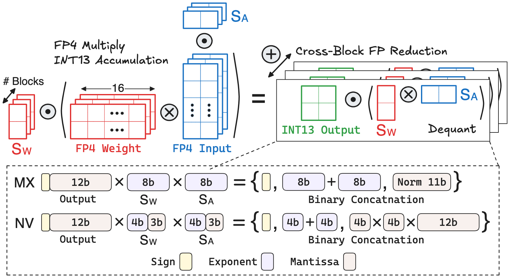
Consider the popular FP4 block-wise quantization under a block size of 16. Let’s analyze the hardware cost of performing block-wise GEMM with the two scale factor quantization approaches:

• Block Dot-product: Since the maximum and minimum FP4 values are \(\pm6\) and \(\pm0.5\), a single FP4 multiplication ranges from \(\pm0.25\) to \(\pm36\), which can be represented using 9-bit fixed-point. With a block size of 16, the dot-product result becomes 13 bits.

• MX Dequantization: To analyze the hardware cost, let’s first write out the binary / decimal values of block scale and dot-product output:

  \[\begin{aligned} \mathrm{S_{W}} &=\, \mathrm{E_{W}} =\, \mathrm{\underbrace{E_{7}\dots E_{0}}_{\text{Exponent}}} \,=\, 2^{\mathrm{E_{W}}-127} \\[0.3em] \mathrm{S_{A}} &=\, \mathrm{E_{A}} =\, \mathrm{\underbrace{E_{7}\dots E_{0}}_{\text{Exponent}}} \,=\, 2^{\mathrm{E_{A}}-127} \\[0.3em] \mathrm{O} \,&=\, \mathrm{S \underbrace{M_{11}\dots M_{0}}_{\text{Un-norm Mantissa}}} =\, (-1)^{\,\mathrm{S}} \cdot \left(\,\Sigma_{j=0}^{11}\,2^{j-2}\cdot\mathrm{M}_{j} \right) \end{aligned}\]

  Based on the above equations, the dequantized output should be:

  \[\mathrm{O_{D}} \,=\, (-1)^{\,\mathrm{S}} \cdot\, 2^{\mathrm{E_{W}} + \mathrm{E_{A}}-254} \cdot \left(\,\underbrace{\Sigma_{j=0}^{11}\,2^{j-2} \cdot \mathrm{M}_{j}}_{\text{Un-norm Mantissa}} \,\right)\]

  Interestingly, this expression has a very similar structure to the standard 32-bit floating-point representation discussed in Section I-2:

  \[\text{FP32} \,=\, \mathrm{\underbrace{S}_{Sign} \; \underbrace{E_7\dots E_{0}}_{\text{Exponent}} \; \underbrace{M_{22}\dots M_{0}}_{\text{Mantissa}}} \,= \,(-1)^{\mathrm{S}} \cdot\, \mathrm{2^{E-127} \cdot 1.{M}}\]

  The dequantized output sign is the FP32 sign, the FP32 exponent \(\mathrm{E} = \mathrm{E_{W}} + \mathrm{E_{A}} - 127\) is calculated via unsigned integer addition, and the FP32 mantissa is obtained via normalizing the dequantized output mantissa. This normalization only requires low-cost hardware components such as Leading-One Detector and Shifter. Finally, the three binary components: sign, exponent, mantissa of dequantized output, are concatenated together (via some simple wiring in hardware) to produce a FP20-E8M11The dequantized output mantissa has 12 bits, but recall the floating-point representation has a hidden mantissa bit that is not stored. number for cross-block partial sum accumulation. To summarize, MX dequantization has low computation cost, involving mainly unsigned integer addition, a leading-one detector, and a shifter.

• NV Dequantization: Again, let’s write out the binary / decimal values of block scale and dot-product output:

  \[\begin{aligned} \mathrm{S_{W}} &=\, \mathrm{\underbrace{E_{3}\dots E_{0}}_{\text{Exponent}} \;\underbrace{M_{2}\dots M_{0}}_{\text{Mantissa}}} \,=\, 2^{\mathrm{E_{W}}-7} \cdot 1.\mathrm{M_{W}} \\[0.3em] \mathrm{S_{A}} &=\, \mathrm{\underbrace{E_{3}\dots E_{0}}_{\text{Exponent}} \;\underbrace{M_{2}\dots M_{0}}_{\text{Mantissa}}} \,=\, 2^{\mathrm{E_{A}}-7} \cdot 1.\mathrm{M_{A}} \\[0.3em] \mathrm{O} \,&=\, \mathrm{S \underbrace{M_{11}\dots M_{0}}_{\text{Un-norm Mantissa}}} =\, (-1)^{\mathrm{S}} \cdot \left(\,\Sigma_{j=0}^{11}\,2^{j-2}\cdot\mathrm{M}_{j} \right) \end{aligned}\]

  Note that the scale factor’s binary encoding does not need the sign bit, as it is always positive by definition of quantization. Based on the above equations, the dequantized output should be:

  \[\mathrm{O_{D}} \,=\, (-1)^{\mathrm{S}} \cdot\, 2^{\mathrm{E_{W}} + \mathrm{E_{A}}-14} \cdot \left[\,1.\mathrm{M_{W}} \cdot 1.\mathrm{M_{A}} \cdot \left(\,\Sigma_{j=0}^{11}\,2^{j-2}\cdot\mathrm{M}_{j}\,\right) \,\right]\]

  Similar to MX, this expression closely matches the standard floating-point representation. The dequantized output sign is the FP sign, and the FP exponent \(\mathrm{E} = \mathrm{E_{W}} + \mathrm{E_{A}} - 14\) is calculated via unsigned integer addition. However, calculating the dequantized output mantissa is more complicated, which involves a 4-bit multiplication between the two scale factors’ mantissa, followed by multiplying the 12-bit output mantissa. Then, the dequantized output mantissa is normalized to the standard FP mantissa via leading-one detector and shifter. Finally, the three binary components: sign, exponent, mantissa of dequantized output, are concatenated together to produce a FP24-E5M19 number for cross-block partial sum accumulation.

Based on the above analysis, the NV dequantizer differs from the MX dequantizer in two notable aspects: (1) It uses a slightly cheaper adder (4-bit vs. 8-bit) for exponent addition; (2) But it requires much more expensive multiplier (\(4\text{-bit} \times 4\text{-bit} \times 12\text{-bit}\)) for mantissa multiplication. Thus, the GEMM hardwareAlso called tensor core in many AI chips. of NV consumes larger area than that of MXFor example, according to this paper from Meta, NVFP4 incurs 12.6% total GEMM hardware area overhead relative to MXFP4, under the same block size of 16..

_{III-3. Hierarchical Scaling for MXFP4}

As discussed in the previous section, NV quantization requires an FP32 tensor scale in addition to the FP8-E4M3 block scale. This multi-level scheme is commonly referred to as hierarchical scaling. The main reason behind NV’s hierarchical scaling is that, the FP8-E4M3 block scale alone may not fully cover a tensor’s dynamic rangeFor example, under NVFP4 quantization, the FP8-E4M3 scale has a dynamic range of [ 2^-9, 448 ]. Multiplying this scale with the FP4 element yields a dynamic range of [ 2^-10, 2688 ], which is insufficient to represent LLM tensors.. On the other hand, MX quantization only requires a single-level block-wise scaling, due to the large dynamic range enabled by its E8M0 block scaleFor example, under MXFP4 quantization, the E8M0 scale has a dynamic range of [ 2^-126, 2¹²⁵ ]. Multiplying this scale with the FP4 element yields a dynamic range of [ 2^-127, 1.5×2¹²⁷ ], which is very close to BF16's dynamic range [ 2^-133, 1.9921875×2¹²⁷ ].. This difference naturally raises the question: Can MX also employ hierarchical scaling? This section presents two case studies from Meta and DeepSeek, demonstrating how hierarchical scaling can enhance MXFP4 to achieve better model accuracy and hardware efficiency.

Meta's MXFP4 Recipe

At first glance, hierarchical scaling may seem unnecessary for MXFP4, since the E8M0 block scale already covers the tensor’s full dynamic range. However, as discussed in Section III-2, one way to reduce the MX quantization error is to bring the mantissa of block maximum closer to that of quantization maximum through additional mantissa scaling, which requires the scale factor to contain mantissa bits. However, directly adding mantissa bits to the E8M0 block scale introduces significant memory and computation overhead during dequantization.

To enable mantissa scaling for MX without sacrificing hardware efficiency, Meta proposes a two-level Macro Block Scaling (MBS) scheme. First, a macro-block (MB) of size \(1 \times 128\) is scaled using an 8-bit mantissa (E0M8), aligning the mantissa of its maximum value close to \(1.5\) (i.e., the mantissa of FP4 maximum). The macro-block is then partitioned into eight local-blocks (LB) of size \(1 \times 16\), each applied MX scaling with an E8M0 block scale. This procedure is visualized below:

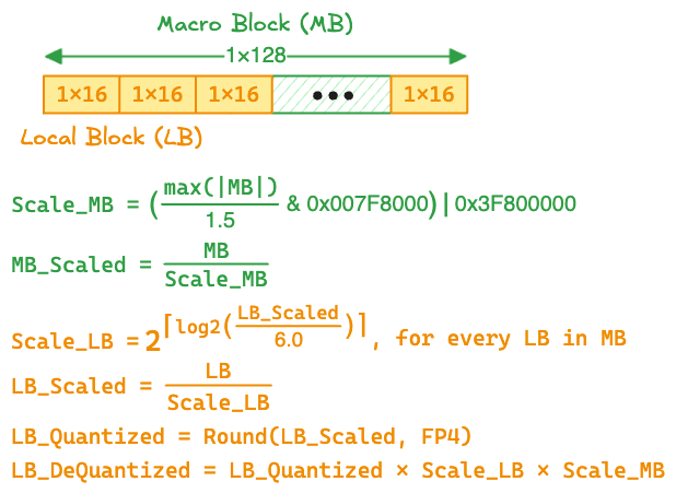
where the E0M8 macro-block scale is obtained by extracting the top 8 mantissa bits of the FP32 scale, i.e., \(\frac{\texttt{max}(\,\mathrm{|MB|}\,)}{1.5} \text{ & 0x007f8000}\).

Why Does MBS Help? Let’s analyze how MBS affects the macro-block maximum, \(\mathrm{B_M}_{\text{max}}\). Assume \(\mathrm{B_M}_{\text{max}}\) is a positive normal FP32 value, leading to the following equations for MBS:

\[\begin{aligned} &\mathrm{B_M}_{\text{max}} = 2^{\mathrm{E'}} \cdot \mathrm{M'} \quad \text{(Assume positive normal value.)} \\[0.1em] &\mathrm{S_{B_M}} = \left(\frac{ \mathrm{B_M}_{\text{max}} }{ 1.5 }\right) = \begin{cases} \; 2^{\mathrm{E'}} \times \left( \frac{\mathrm{M'}}{1.5} \right) & \text{if } \mathrm{M'} \geq 1.5 \\[0.1em] \; 2^{\mathrm{E'}-1} \times \left( \frac{\mathrm{M'}}{1.5} \cdot 2 \right) & \text{if } \mathrm{M'} < 1.5 \end{cases} \\[0.3em] &\text{(Assume retaining the top 8 bits can sufficiently preserve the whole mantissa.)} \\ &\mathrm{S_{B_M}} = \begin{cases} \; \frac{\mathrm{M'}}{1.5} & \text{if } \mathrm{M'} \geq 1.5 \\[0.1em] \; \frac{\mathrm{M'}}{1.5} \cdot 2 & \text{if } \mathrm{M'} < 1.5 \end{cases} \\[0.3em] &\mathrm{B_{M,\,S}} = \frac{\mathrm{B_M}}{\mathrm{S_{B_M}}} = \begin{cases} \; 2^{\mathrm{E'}} \cdot 1.5 & \text{if } \mathrm{M'} \geq 1.5 \\[0.1em] \; 2^{\mathrm{E' - 1}} \cdot 1.5 & \text{if } \mathrm{M'} < 1.5 \end{cases} \\[0.3em] \end{aligned}\]

The above analysis assumes that retaining the top 8 mantissa bits is sufficient to preserve the whole mantissa, which is generally true. Empirically, Meta finds that the top 8 mantissa bits can approximate the original FP32 mantissa with \(<0.3\%\) error. After performing MBS, the scaled maximum \(\mathrm{B_{M,\,S}}\) has a mantissa of \(1.5\), which can be accurately quantized to 6.0 during the MXFP4 quantization of local-blocks.

The benefits of MBS is two fold. First, it enables more accurate quantization of the macro-block maximum, thereby preserving the numerical fidelity of many high-magnitude outliers. Second, the \(1 \times 128\) macro-block size significantly reduces the memoryEach macro-block of 128 elements store an 8-bit E0M8 scale, while each local-block of 16 elements store an 8-bit E8M0 scale. Under FP4 quantization, this gives an effective memory cost of (4 + 8/16 + 8/128) = 4.5625 bits per element. In practice, the memory cost can be further reduced by packing the 8-bit macro-block scale within the local-block scales, since an E7M0 local-block scale is sufficient to cover the tensor's dynamic range. and dequantization cost compared to allocating extra mantissa bits to the local-block scale.

To quantify the algorithmic benefits of MBS, I implement Meta’s MXFP4 quantizerIn addition to MBS, Meta's MXFP4 also proposes a technique called Overflow-Aware Scaling (OBS), which I don't cover in this blog but is implement in the quantizer. and compare it with the baseline MXFP4 quantizer discussed in Section III-2. The following table shows the perplexity of Wikitext-2 dataset on several Llama3 and Qwen3 models, under MXFP4 weight-activation quantization with a block size of 16. Meta’s recipe achieves much better perplexity compared to the baseline MXFP4 quantization.

	Llama-3.1-8B	Llama-3.2-3B	Qwen3-4B	Qwen3-8B
Baseline MXFP4	8.69	13.58	15.69	10.66
Meta's MXFP4	8.14	12.82	14.52	10.42

Hardware Implication of MBS: While Meta claims that MBS does not require any change to the GEMM hardware (tensor core), it still necessitates a careful architecture co-design to balance the throughput between tensor core and vector core. Below is a visualization of the GEMM computation flow using MBS:

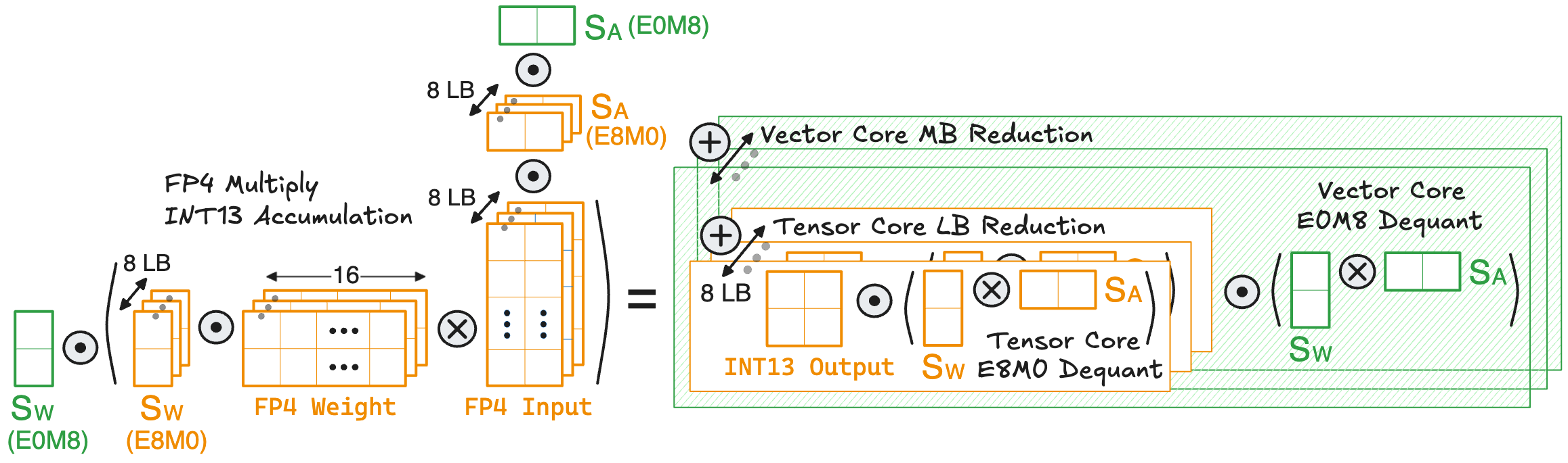
Within a macro-block, the eight local-blocks are all quantized to MXFP4. Therefore, the macro-block dot product, comprising 128 MAC operations, can be accelerated using the dedicated MXFP4 tensor core. However, the macro-block output must be dequantized by multiplying it with two E0M8 scales, followed by accumulation across different macro-blocks. This process is realized on the FP32 vector core and involves 2 MAC operationsTechnically, the macro-block dequantization involves 1 multiplication between the two E0M8 scales and 1 MAC with the macro-block output. However, most AI hardware performs fused MAC operations in a single cycle; if only a multiplication or addition is issued, the other part of the MAC unit becomes idle.. In order to fully utilize the MXFP4 tensor core for GEMM, the vector core throughput should exceed \(1/64\) of the tensor core throughputThis requirement may not be met on some existing GPUs. For example, on NVIDIA GB300 NVL72, the FP32 vector core throughput is only 1/180 of the FP4 tensor core throughput..

DeepSeek's MXFP4 Recipe

The recent DeepSeek-V4 adopts mixed-precision quantization for the mixture-of-expert layers, where weights and activations are quantized to MXFP4 and MXFP8The mixed-precision configuration using 4-bit weights and 8-bit activations is commonly referred to as W4A8 quantization., respectively, with block sizes of 32 and 128. However, mainstream AI hardware typically requires both GEMM inputs to use the same numerical precision, forcing the lower-precision operand (FP4 weights in this case) to be first upcast to the higher precision (FP8 in this case) before GEMM can be performed. Consider an example GEMM tile size of \(128 \times 128 \times 1\), which is the default tile size used in DeepSeek-V3. The naive mixed-precision GEMM flow is visualized below:

Since each \(1 \times 32\) weight block has its own E8M0 scale, the tensor core can only perform a 32-way FP8 dot product, after which the output must be dequantized on the vector coreIn recent AI hardware such as NVIDIA Blackwell and AMD Instinct GPUs, the MX tensor core natively supports E8M0 dequantization with a block size of 32. Thus, I believe this straightforward GEMM flow can work efficiently on the latest GPUs.. However, as highlighted in DeepSeek-V4’s technical report, performing a full 128-way dot-product (without intermediate dequantization) on the FP8 tensor core allows to reuse DeepSeek-V3’s existing FP8 training framework without modificationTherefore, the hierarchical MXFP4 scaling in DeepSeek-V4, which will be described next, is primarily an engineering design choice. But it's still a very smart technique..

To enable a complete \(128 \times 128 \times 1\) FP8 GEMM between weights and activations, all dequantized weight blocks within a \(128 \times 128\) tile should be representable in FP8, which leads to a tile-wise MX scaling as described in the following equations:

\[\begin{aligned} &\text{For every } \mathrm{B} \text{ in } \mathrm{T}: \\[0.3em] &\quad\;\; \mathrm{S}_\text{B} = \frac{ |\mathrm{B}|_{\text{max}} }{ 6 } ; \ \ \mathrm{S_{Q}} = 2^{\left\lceil\,\texttt{log2}\left( \,\mathrm{S}_\text{B} \,\right) \,\right\rceil} ; \ \ \mathrm{B_{S}} = \frac{\mathrm{B}}{\mathrm{S_{Q}}} \quad\quad \text{(Original MXFP4 Scaling)} \\[0.3em] &\quad\;\; \mathrm{B_{Q}} = \texttt{Round}\left(\,\mathrm{B_{S}}\,,\, \text{FP4}\,\right) \quad\;\;\, \text{(Quantized FP4 Block)} \\[0.3em] &\mathrm{S}_\text{T} = \frac{\texttt{max}\left(\,\mathrm{S_{Q}}\,\right)}{64} \quad\quad \text{(E8M0 Tile Scale)} \\[0.3em] &\text{For every } \mathrm{B} \text{ in } \mathrm{T}: \\[0.3em] &\quad\;\; \mathrm{S}_\text{B} = \frac{\mathrm{S_{Q}}}{\mathrm{S}_\text{T}} \quad\quad\quad\,\, \text{(E8M0 Block scale; Store in E4M0)} \\[0.3em] &\quad\;\; \mathrm{B_D} = \mathrm{B_Q} \cdot \mathrm{S_B} \quad\;\; \text{(Dequantized FP8 block for GEMM)} \\[0.3em] &\mathrm{T_D} = \mathrm{B_D} \cdot \mathrm{S_{T}} \quad\quad\;\;\;\; \text{(Dequantized Tile after FP8 GEMM)} \end{aligned}\]

where \(\mathrm{T}\) and \(\mathrm{B}\) denote the \(128 \times 128\) weight tile and the \(1 \times 32\) weight block, respectively. \(\mathrm{S}_\text{T}\) and \(\mathrm{S}_\text{B}\) denote the tile scale and block scale, respectively. The subscripts \(_{\text{S}\,}\), \(_{\text{Q}\,}\), and \(_{\text{D}\,}\) represent the scaled, quantized, and dequantized operand, respectively.

There are several important details in the above recipe that are worth discussing:

• When computing the tile scale \(\mathrm{S_{T}}\), where does the magic number \(64\) come from? It is to ensure the block scale \(\mathrm{S_B} \leq 64\) and the dequantized block \(\mathrm{B_D} \leq 6 \times 64 = 384\), which maximizes the utilization of FP8 quantization valuesFor example, choosing $$\mathrm{S_T} = \frac{\text{max}(\mathrm{S_Q})}{128} \implies \mathrm{B_D} < 768$$which may exceed the maximum FP8 value. Similarly, choosing $$\mathrm{S_T} = \frac{\text{max}(\mathrm{S_Q})}{32} \implies \mathrm{B_D} ≤ 192$$which can waste many FP8 quantization values. You may want to use some example tensors and try this out in Pytorch for better visualization..
• When computing the block scale \(\mathrm{S_{B}}\), I leave a note saying that it can be stored in E4M0, which has a power-of-two range \([\,2^{-6}, 2^8\,]\). This allows the dequantized block \(\mathrm{B_D} = \mathrm{B_Q} \cdot \mathrm{S_{B}}\) to be perfectly represented in FP8-E4M3 without overflow and underflow. But does E4M0 introduce extra error compared to the original E8M0 block scale? As discussed in the previous point, \(\mathrm{S_B} \leq 64 = 2^6\) already falls within the upper bound of E4M0. The remaining concern is whether the smallest block scale is guaranteed to be larger than \(2^{-6}\). Empirically, DeepSeek finds that their model weights satisfy this conditionI believe this condition holds for most LLMs. In general, prior work has observed that LLM weights tend to exhibit a small dynamic range, meaning their binary exponents have small difference and can be encoded with fewer bits..

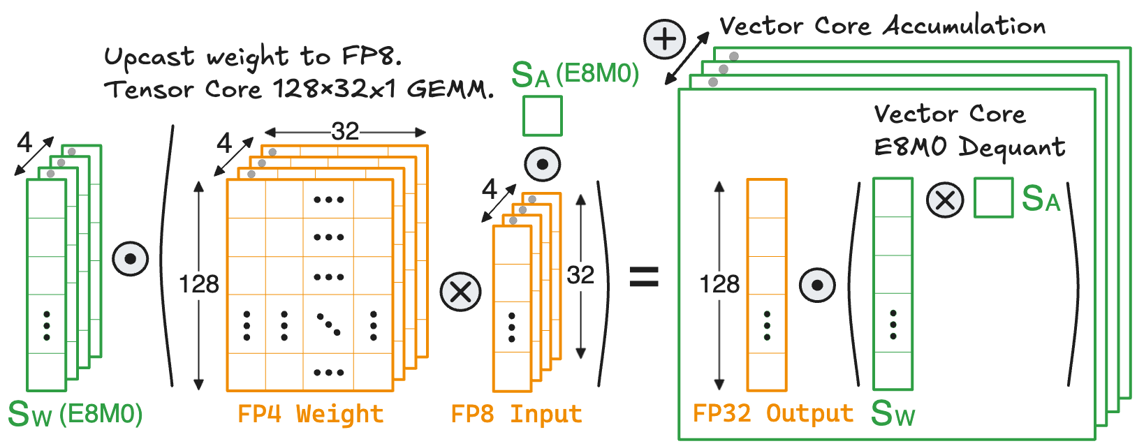
Hardware Implication: With DeepSeek’s hierarchical MXFP4 scaling, the \(128 \times 128 \times 1\) mixed-precision GEMM flow becomes:

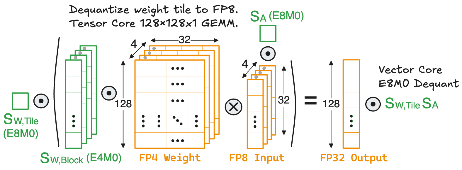
Now, the entire \(128 \times 128\) weight tile can be first dequantized to FP8, where each \(1 \times 32\) weight block is multiplied by its E4M0 block scale. Then a \(128 \times 128 \times 1\) FP8 GEMM is performed on the tensor core. Finally, the GEMM output is dequantized on the vector core by multiplying it with the two scales of weight tile and activation block.

Let’s analyze the computation cost of dequantization before and after applying DeepSeek’s hierarchical scaling. In the naive GEMM with single-level MXFP4 scaling, the vector core performs 1024 multiplicationsUnder a more efficient hardware implementation, these multiplications can become 8-bit exponent addition since the scale factors are E8M0. and 512 accumulations. Whereas in the new GEMM with hierarchical scaling, only (128 + 1) multiplications and 128 accumulationsAlthough these accumulations are not shown in the above figure, they are required when the full LLM dot-product size is larger than 128..

Acknowledgment

• Special thanks to Xilai Dai (Cornell University), Dr. Chao Fang (KU Leuven), and Prof. Mohamed Abdelfattah (Cornell University), for helping shape out the content of this blog.
• For readers with a broad interest in Machine Learning Hardware and Systems, my advisor Mohamed Abdelfattah has a nice lecture series available on his website and Youtube.
• I decided to write this blog partly because I stumbled over Simon Boehm’s amazing blog about CUDA Matmul kernel optimization.
• Drawings are largely made with Excalidraw.